My notes on "A guide to convolution arithmetic for deep learning"
Vincent Dumoulin and Francesco Visin. “A Guide to Convolution Arithmetic for Deep Learning.” arXiv preprint arXiv:1603.07285, 2016. https://arxiv.org/abs/1603.07285
Diagrams drawn with Excalidraw.
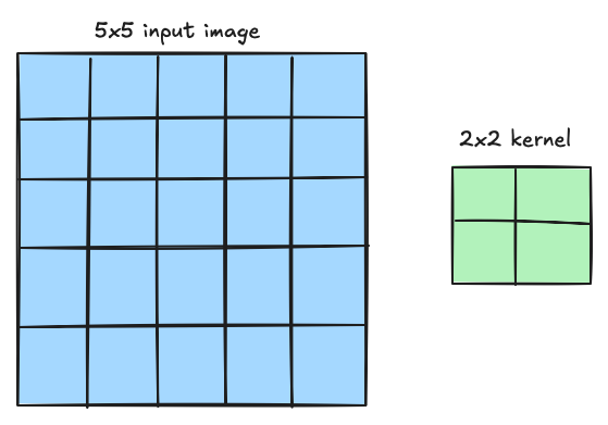
Setup: Input and Kernel
We start with a $5 \times 5$ input image and a $2 \times 2$ kernel.
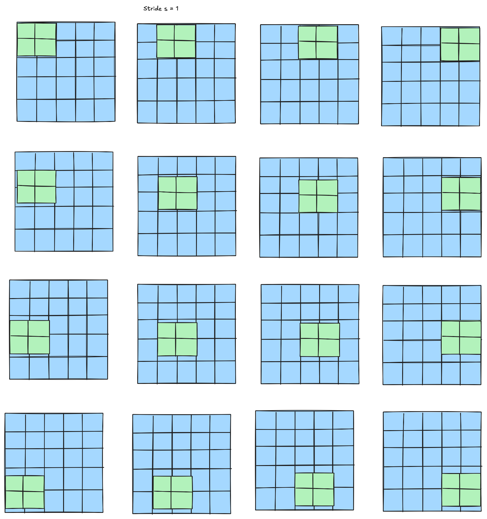
Convolution with Stride $s = 1$
The $2 \times 2$ kernel slides across the $5 \times 5$ input with stride $s = 1$, visiting all 16 positions ($4 \times 4$ grid) from top-left to bottom-right.
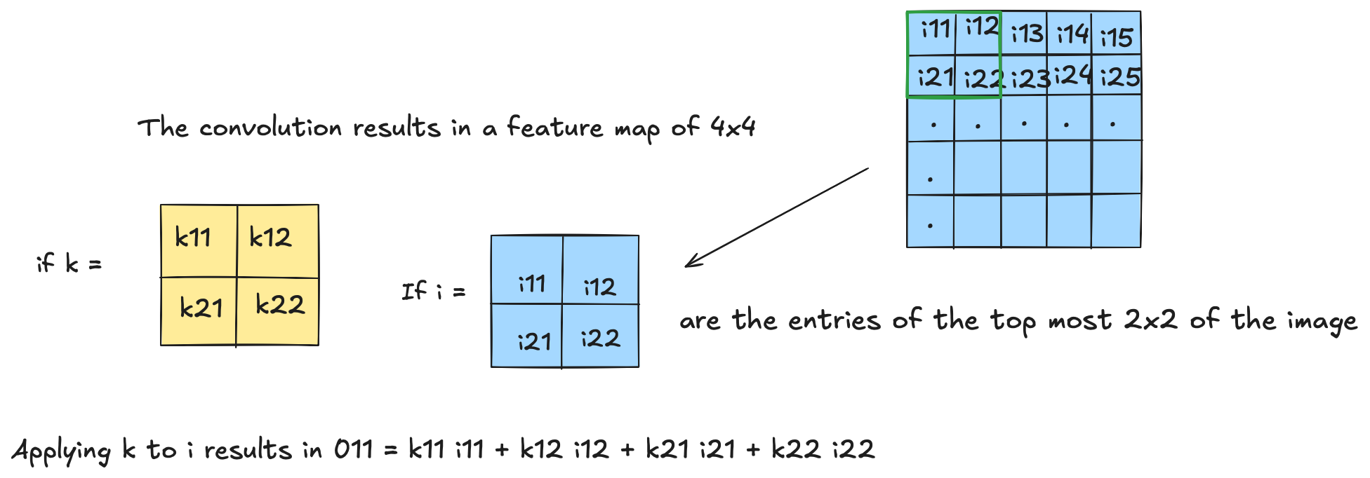
Computing one output value. Let
$$K = \begin{pmatrix} k_{11} & k_{12} \\ k_{21} & k_{22} \end{pmatrix}, \qquad I = \begin{pmatrix} i_{11} & i_{12} \\ i_{21} & i_{22} \end{pmatrix}$$where $I$ contains the entries of the top-left $2 \times 2$ patch of the image. Applying $K$ to $I$ gives:
$$O_{11} = k_{11}\,i_{11} + k_{12}\,i_{12} + k_{21}\,i_{21} + k_{22}\,i_{22}$$The convolution results in a feature map of size $4 \times 4$.
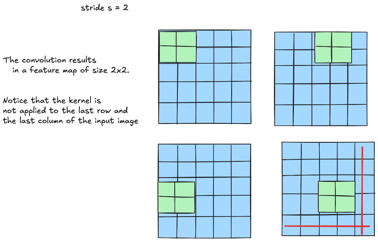
Convolution with Stride $s = 2$
With stride $s = 2$, the kernel jumps two pixels at a time. The convolution results in a feature map of size $2 \times 2$.
Note: the kernel is not applied to the last row and the last column of the input image.
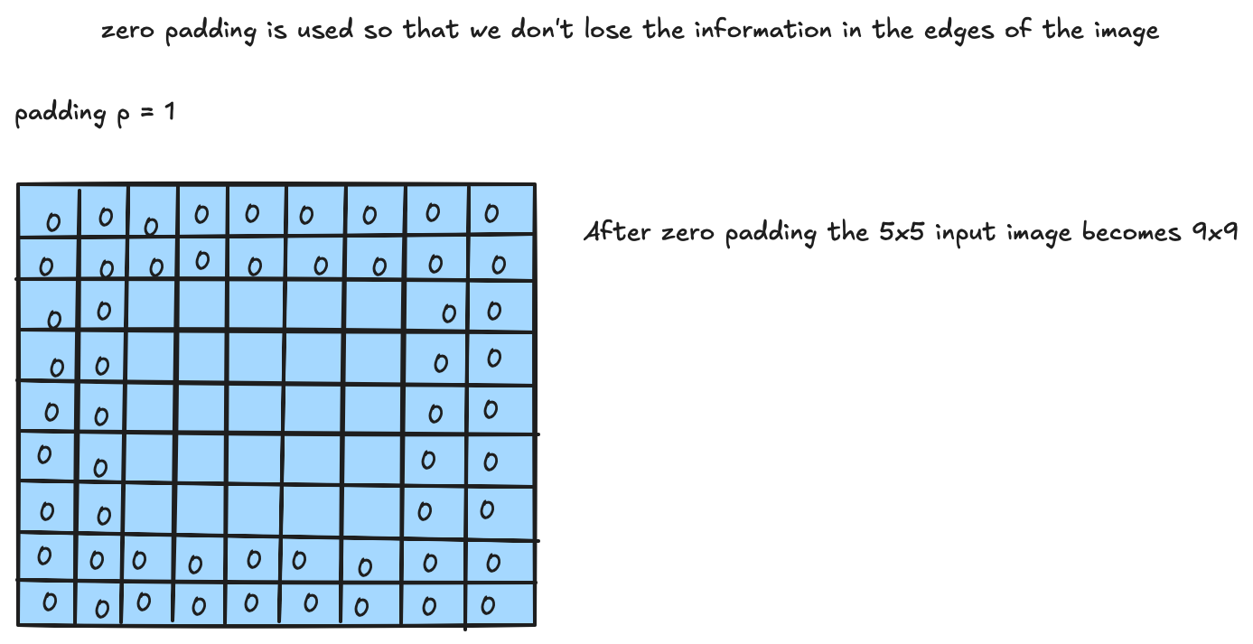
Zero Padding
Zero padding is used so that we don’t lose the information at the edges of the image.
With padding $p = 1$, the $5 \times 5$ input becomes $7 \times 7$ after padding. In general, with padding $p$, the image grows to $(i + 2p) \times (i + 2p)$.
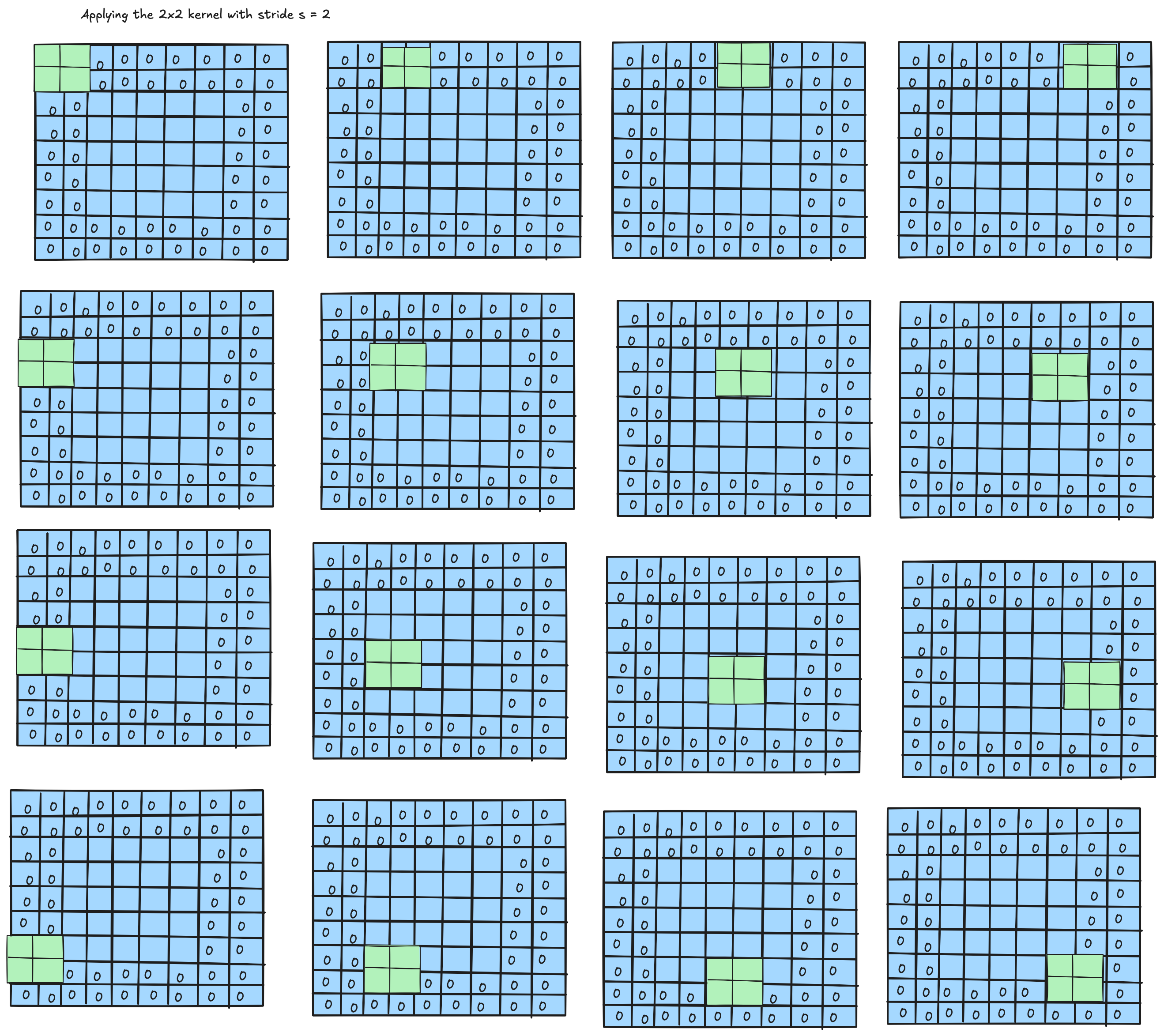
Applying the $2 \times 2$ kernel with stride $s = 2$ to the zero-padded image:
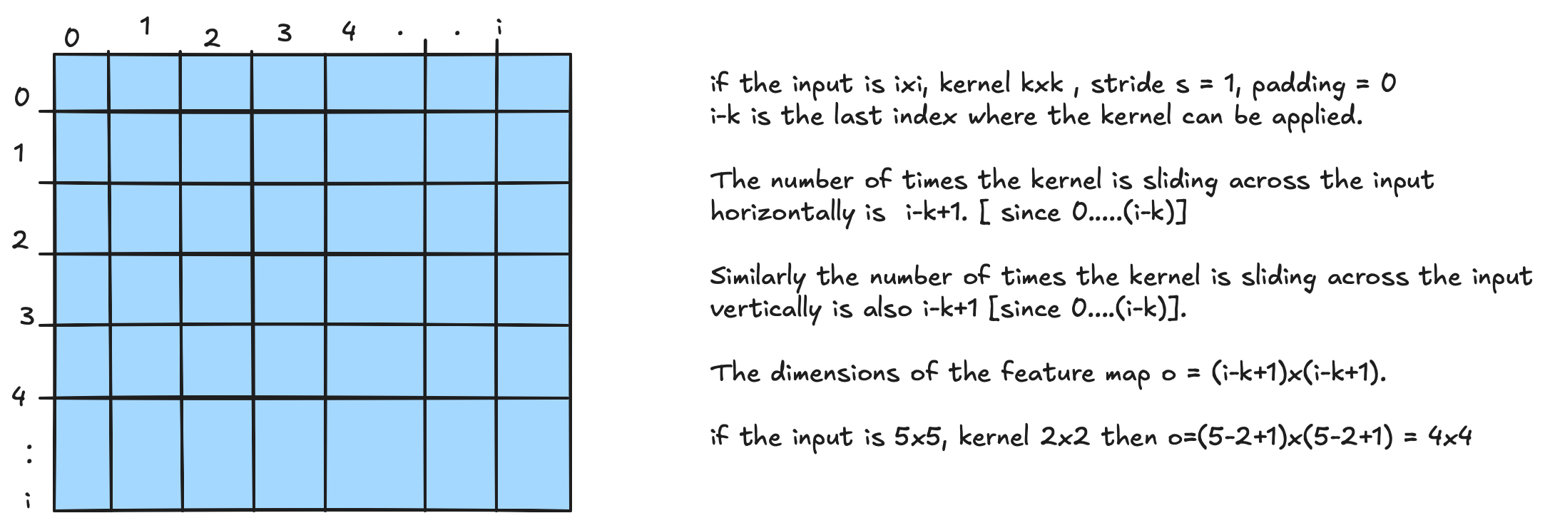
Feature Map Size Formula (no padding, $s = 1$)
For an $i \times i$ input, $k \times k$ kernel, stride $s = 1$, and padding $p = 0$:
- $i - k$ is the last index where the kernel can be applied.
- The number of times the kernel slides horizontally is $i - k + 1$ (indices $0, 1, \ldots, i-k$).
- The same holds vertically.
Example: $5 \times 5$ input, $2 \times 2$ kernel $\Rightarrow o = (5 - 2 + 1)^2 = 4 \times 4$.
Feature Map Size Formula (with padding, $s = 1$)
With stride $s = 1$ and non-zero padding $p$, the padded image has size $i + 2p$, so the kernel slides $(i + 2p) - k + 1$ times in each direction:
$$\boxed{o = (i + 2p - k + 1) \times (i + 2p - k + 1)}$$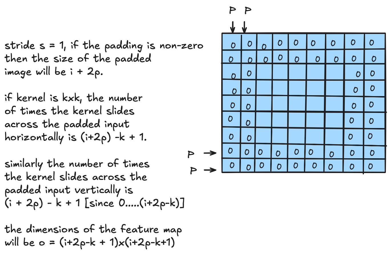
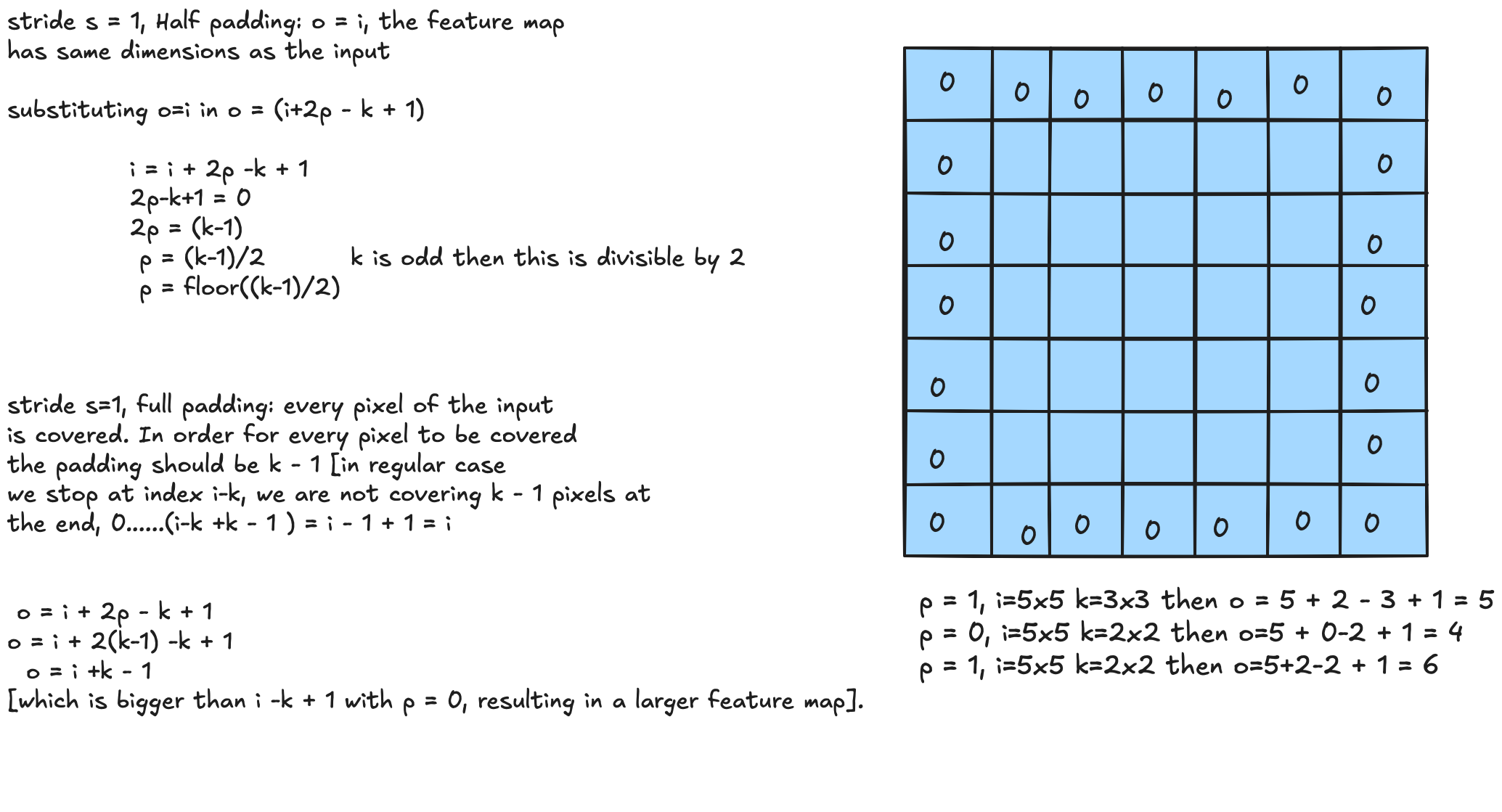
Special Padding Cases ($s = 1$)
Half Padding
The feature map has the same dimensions as the input: $o = i$.
Substituting $o = i$ into $o = i + 2p - k + 1$:
$$i = i + 2p - k + 1 \implies 2p = k - 1 \implies p = \frac{k-1}{2}$$When $k$ is odd this is an integer; in general $p = \lfloor (k-1)/2 \rfloor$.
Full Padding
Every pixel of the input is visited as the first element of some patch. Without padding the last kernel position is $i - k$, so the first $k - 1$ pixels of the input are never a patch’s starting element. Setting $p = k - 1$ lets the kernel start at $-(k-1)$, fixing that:
$$o = i + 2(k-1) - k + 1 = i + k - 1$$This produces a larger feature map than the $p = 0$ case.
Examples:
| $p$ | Input | Kernel | $o$ |
|---|---|---|---|
| 1 | $5 \times 5$ | $3 \times 3$ | $5 + 2 - 3 + 1 = 5$ |
| 0 | $5 \times 5$ | $2 \times 2$ | $5 + 0 - 2 + 1 = 4$ |
| 1 | $5 \times 5$ | $2 \times 2$ | $5 + 2 - 2 + 1 = 6$ |
Feature Map Size Formula (stride $s > 1$)
The last index covered is $i - k$. With stride $s > 1$ and no padding:
$$o = \left\lfloor \frac{i - k}{s} \right\rfloor + 1$$With non-zero padding:
$$\boxed{o = \left\lfloor \frac{i + 2p - k}{s} \right\rfloor + 1}$$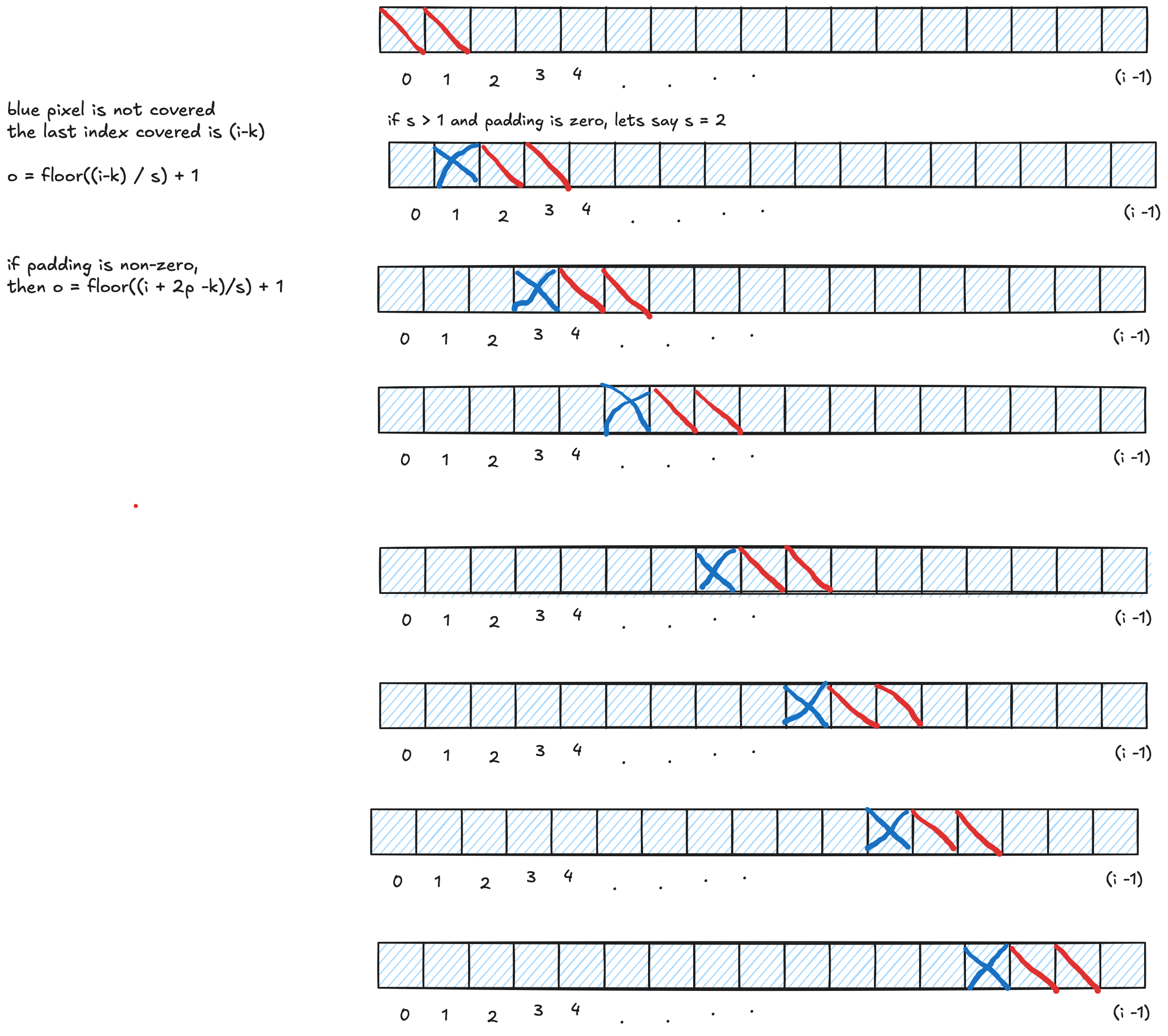
Multi-Channel (RGB) Convolution
For an RGB image, the same kernel is applied to each channel independently, producing feature maps $C_1$, $C_2$, $C_3$. The combined output is:
$$C = C_1 + C_2 + C_3$$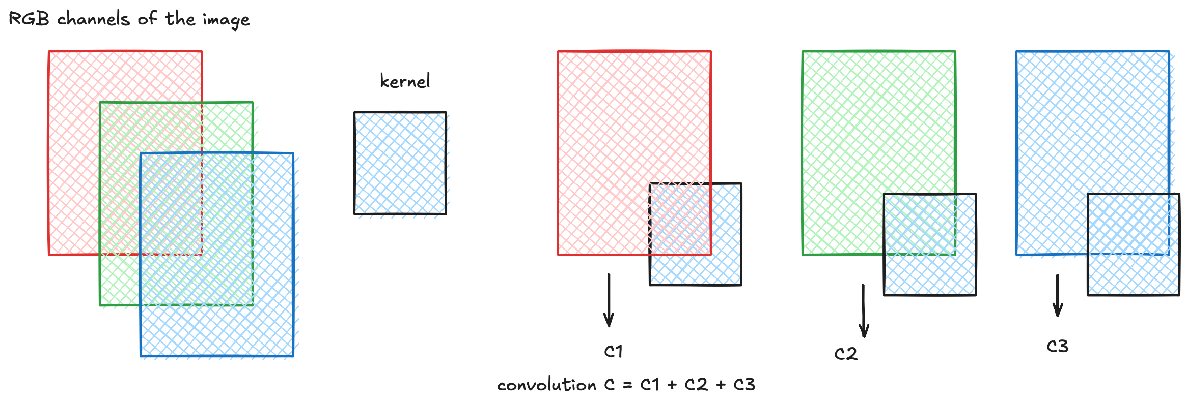
Pooling
Pooling achieves translation invariance. Two common types:
- Max pooling (stride $s = 2$): takes the maximum pixel value from each $k \times k$ region.
- Average pooling (stride $s = 2$): takes the average of all pixels in each $k \times k$ region.
The output size formula is the same as convolution with $p = 0$:
$$o = \left\lfloor \frac{i - k}{s} \right\rfloor + 1$$Example ($4 \times 4$ input, $2 \times 2$ pool, $s = 2$):
$$\text{Max pooling} = \begin{pmatrix} 6 & 8 \\ 14 & 16 \end{pmatrix} \qquad \text{Average pooling} = \begin{pmatrix} 3.5 & 5.5 \\ 11.5 & 13.5 \end{pmatrix}$$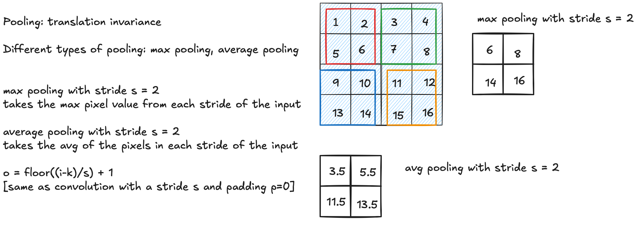
Convolution as Matrix Multiplication
Consider a $4 \times 4$ input $A$, $2 \times 2$ kernel $W$, and stride $s = 2$:
$$A = \begin{pmatrix} a_{11} & a_{12} & a_{13} & a_{14} \\ a_{21} & a_{22} & a_{23} & a_{24} \\ a_{31} & a_{32} & a_{33} & a_{34} \\ a_{41} & a_{42} & a_{43} & a_{44} \end{pmatrix}, \qquad W = \begin{pmatrix} w_{11} & w_{12} \\ w_{21} & w_{22} \end{pmatrix}$$Flatten each $2 \times 2$ patch (left-to-right, top-to-bottom) into a row, and flatten the kernel into a column vector $\mathbf{w} = (w_{11}, w_{12}, w_{21}, w_{22})^\top$:
$$\begin{pmatrix} a_{11} & a_{12} & a_{21} & a_{22} \\ a_{13} & a_{14} & a_{23} & a_{24} \\ a_{31} & a_{32} & a_{41} & a_{42} \\ a_{33} & a_{34} & a_{43} & a_{44} \end{pmatrix} \begin{pmatrix} w_{11} \\ w_{12} \\ w_{21} \\ w_{22} \end{pmatrix} = \begin{pmatrix} a_{11}w_{11} + a_{12}w_{12} + a_{21}w_{21} + a_{22}w_{22} \\ a_{13}w_{11} + a_{14}w_{12} + a_{23}w_{21} + a_{24}w_{22} \\ a_{31}w_{11} + a_{32}w_{12} + a_{41}w_{21} + a_{42}w_{22} \\ a_{33}w_{11} + a_{34}w_{12} + a_{43}w_{21} + a_{44}w_{22} \end{pmatrix}$$Reshaping this $4 \times 1$ result as $2 \times 2$ gives the feature map:
$$\text{feature map} = \begin{pmatrix} a_{11}w_{11}+a_{12}w_{12}+a_{21}w_{21}+a_{22}w_{22} & a_{13}w_{11}+a_{14}w_{12}+a_{23}w_{21}+a_{24}w_{22} \\ a_{31}w_{11}+a_{32}w_{12}+a_{41}w_{21}+a_{42}w_{22} & a_{33}w_{11}+a_{34}w_{12}+a_{43}w_{21}+a_{44}w_{22} \end{pmatrix}$$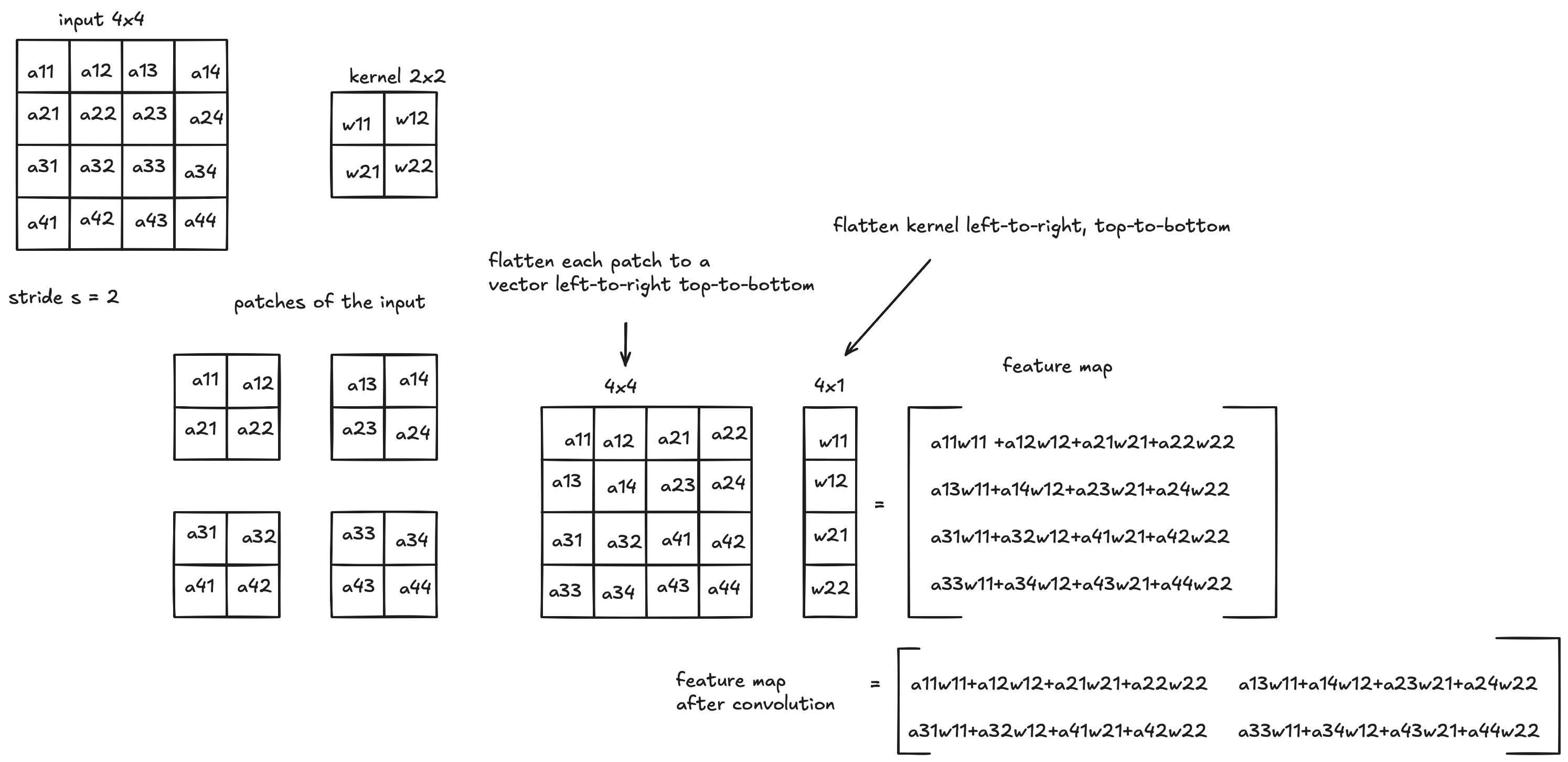
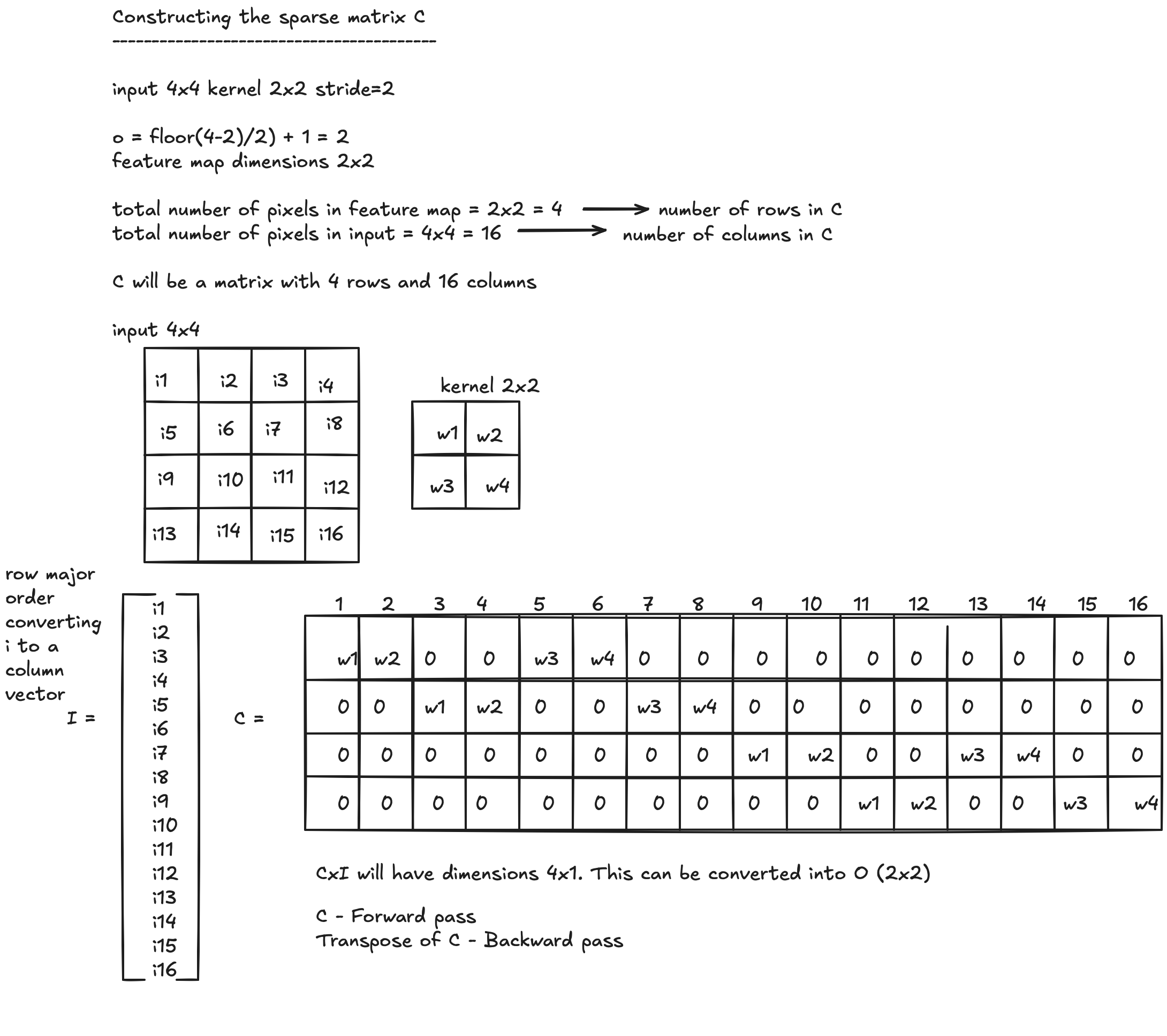
The Sparse Matrix $C$
Setup: $4 \times 4$ input, $2 \times 2$ kernel, stride $s = 2$.
$$o = \left\lfloor \frac{4-2}{2} \right\rfloor + 1 = 2 \quad \Rightarrow \quad \text{feature map is } 2 \times 2$$- Total pixels in feature map $= 2 \times 2 = 4$ → number of rows in $C$
- Total pixels in input $= 4 \times 4 = 16$ → number of columns in $C$
So $C$ is a $4 \times 16$ sparse matrix:
$$C = \begin{pmatrix} w_1 & w_2 & 0 & 0 & w_3 & w_4 & 0 & 0 & 0 & 0 & 0 & 0 & 0 & 0 & 0 & 0 \\ 0 & 0 & w_1 & w_2 & 0 & 0 & w_3 & w_4 & 0 & 0 & 0 & 0 & 0 & 0 & 0 & 0 \\ 0 & 0 & 0 & 0 & 0 & 0 & 0 & 0 & w_1 & w_2 & 0 & 0 & w_3 & w_4 & 0 & 0 \\ 0 & 0 & 0 & 0 & 0 & 0 & 0 & 0 & 0 & 0 & w_1 & w_2 & 0 & 0 & w_3 & w_4 \end{pmatrix}$$$C \cdot I$ (where $I$ is the input flattened in row-major order) has dimensions $4 \times 1$, which reshapes to the output $O$ ($2 \times 2$).
- $C$ is used in the forward pass
- $C^\top$ is used in the backward pass
Transposed Convolution
- Convolution: downsampling
- Transposed convolution: upscaling
Using the same $4 \times 4$ input, $2 \times 2$ kernel, stride $s = 2$, the feature map $O$ is $2 \times 2$, flattened as $O = (a,\, b,\, c,\, d)^\top$.
The transpose $C^\top$ has dimensions $16 \times 4$. The upscaled feature map is:
$$C^\top \cdot O = \begin{pmatrix} w_1 a \\ w_2 a \\ w_1 b \\ w_2 b \\ w_3 a \\ w_4 a \\ w_3 b \\ w_4 b \\ w_1 c \\ w_2 c \\ w_1 d \\ w_2 d \\ w_3 c \\ w_4 c \\ w_3 d \\ w_4 d \end{pmatrix}$$Reshaped as $4 \times 4$:
$$\begin{pmatrix} w_1 a & w_2 a & w_1 b & w_2 b \\ w_3 a & w_4 a & w_3 b & w_4 b \\ w_1 c & w_2 c & w_1 d & w_2 d \\ w_3 c & w_4 c & w_3 d & w_4 d \end{pmatrix}$$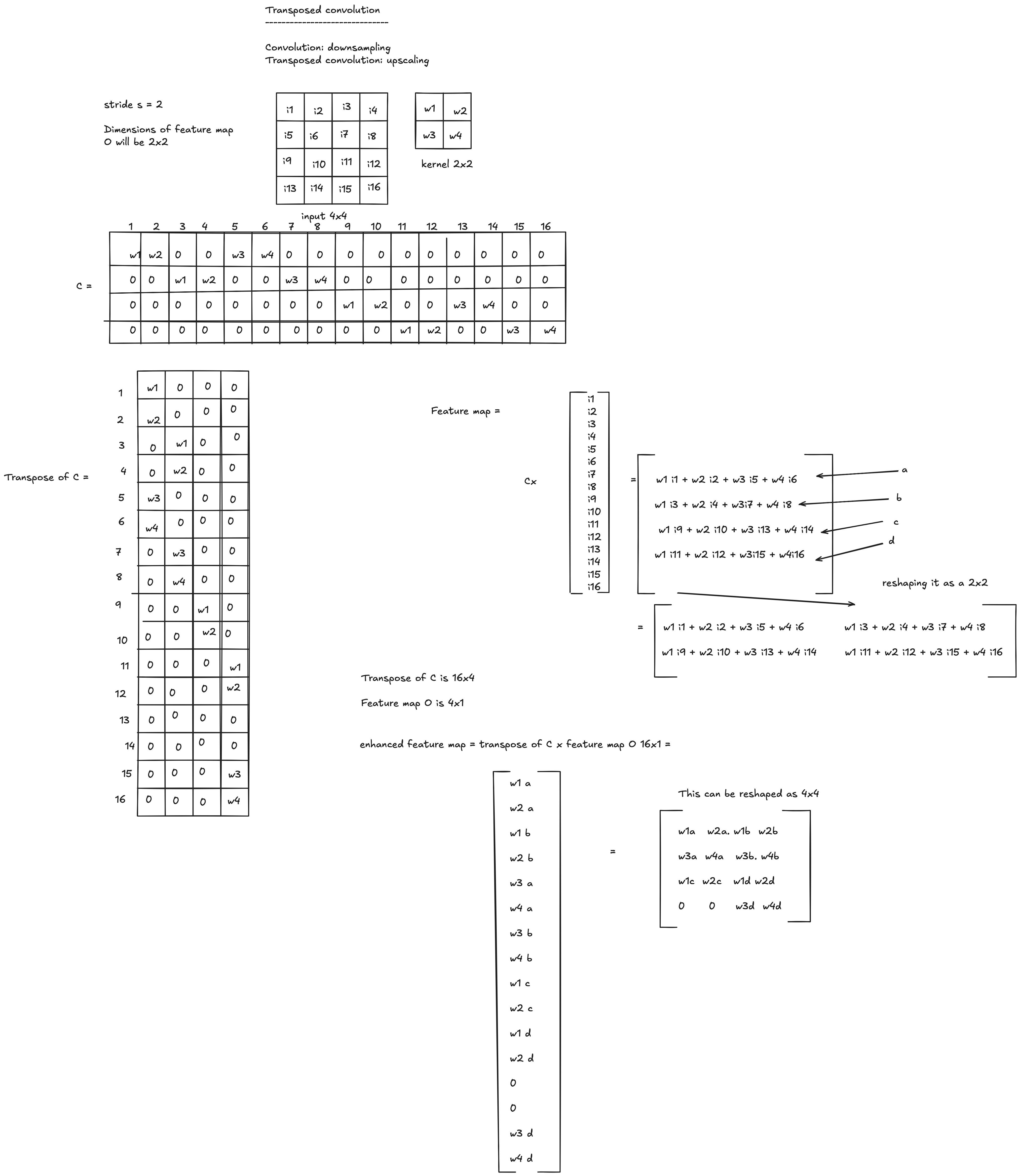
Transposed Convolution Output Size
Let $[a\ b\ c]$ be the input. Each element is expanded by applying the kernel, and results are accumulated with overlaps determined by the stride.
-
$k=3$, $s=1$, $p=0$: Since $s < k$, there is a $k - s = 2$ overlap between blocks.
$$a_1\ (a_2+b_1)\ (a_3+b_2+c_1)\ (b_3+c_2)\ c_3 \qquad \text{output size} = 5$$ -
$k=3$, $s=3$, $p=0$: Since $s = k$, there is no overlap.
$$a_1\ a_2\ a_3\ b_1\ b_2\ b_3\ c_1\ c_2\ c_3 \qquad \text{output size} = 9$$ -
$k=3$, $s=4$, $p=0$: Since $s > k$, zeros are inserted between blocks.
$$a_1\ a_2\ a_3\ 0\ b_1\ b_2\ b_3\ 0\ c_1\ c_2\ c_3 \qquad \text{output size} = 11$$ -
$k=3$, $s=3$, $p=2$: Expand to $a_1\,a_2\,a_3\,b_1\,b_2\,b_3\,c_1\,c_2\,c_3$, then remove the first and last $p=2$ elements (which interacted with padded zeros): $a_3\ b_1\ b_2\ b_3\ c_1$, output size $= 5$.
In general:
$$\boxed{o' = s(i - 1) + k - 2p}$$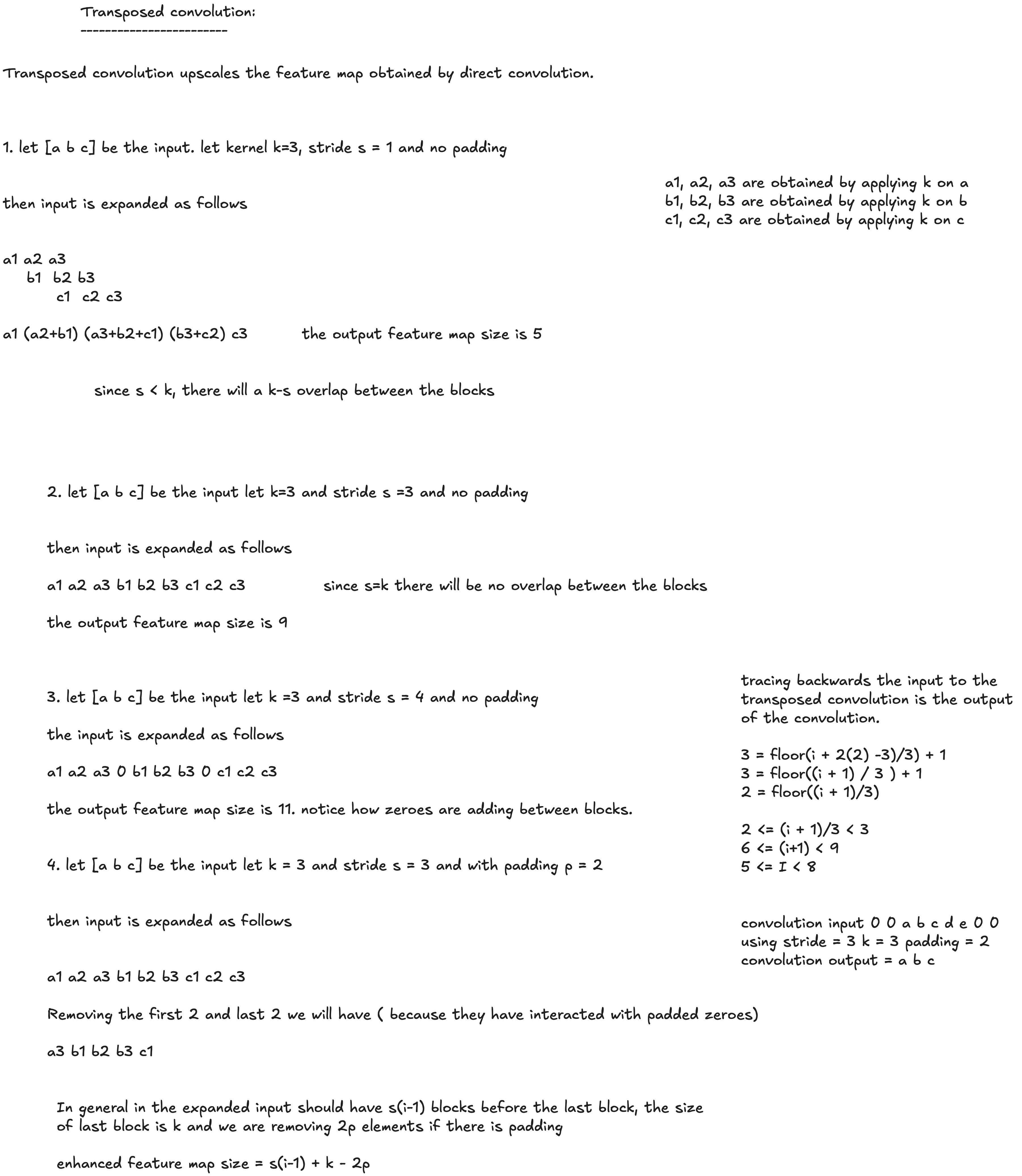
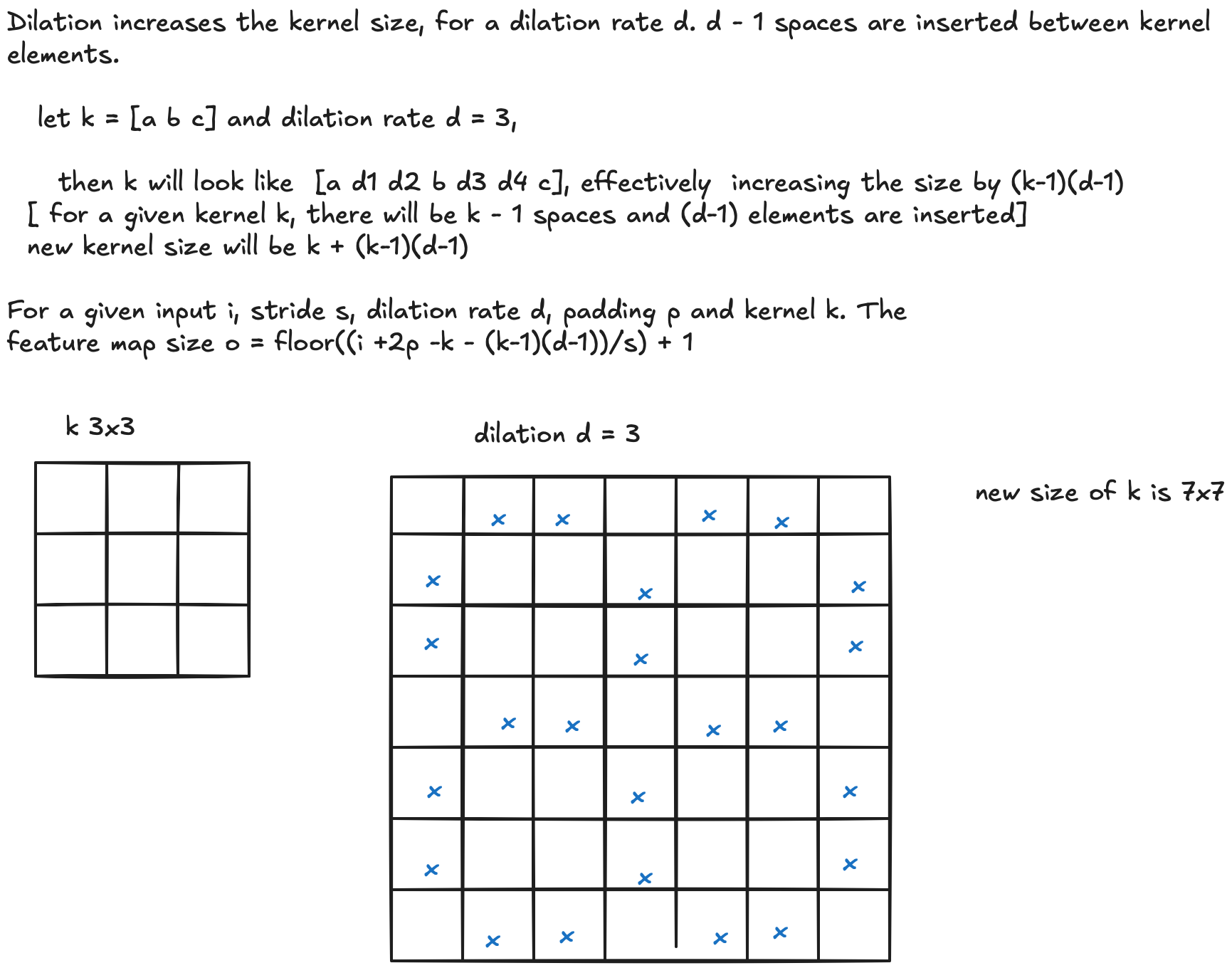
Dilated Convolution
Dilation increases the effective kernel size. For a dilation rate $d$, $(d-1)$ zeros are inserted between each pair of kernel elements.
Example: let $k = [a\ b\ c]$ and $d = 3$. The dilated kernel becomes $[a\ d_1\ d_2\ b\ d_3\ d_4\ c]$, effectively increasing the size by $(k-1)(d-1)$.
New kernel size:
$$k' = k + (k-1)(d-1)$$For input $i$, stride $s$, dilation rate $d$, padding $p$, kernel $k$:
$$\boxed{o = \left\lfloor \frac{i + 2p - k - (k-1)(d-1)}{s} \right\rfloor + 1}$$Example: a $3 \times 3$ kernel with dilation $d = 3$ becomes a $7 \times 7$ dilated kernel (with zeros at non-kernel positions).